gdr3binaryorbits

Python code to visualize the radial velocity orbits published in Gaia DR3.

Note: Currently only supports queries for SB1 orbits. SB2 orbits will be added shortly!

Details on the NSS orbits: Gaia DR3 NSS_TWO_BODY_ORBIT Documentation

Installation

1. Clone the repo

   git clone https://github.com/tjayasinghe/gdr3binaryorbits.git

2. Install with python

   python setup.py install

(back to top)

Usage

Here is an example on how to use this project to retrieve and visualize an SB1 RV orbit published in Gaia DR3.

1. Create a NSS object

   from gdr3binaryorbits.orbits import NSS
   
   star=NSS()

2. A star can be loaded either through a cone search with RAJ2000 and DEJ2000 coordinates or through a direct query based on the Gaia DR3 source_id.

   star.query_source('5853193426917488128') #Query by source_id
   star.query_coords(219.41107637177004,-63.36791102568197) #Cone search

3. Once the star is loaded, query the Gaia DR3 NSS database and search for a SB1 orbit.

   star.query_nss('SB1')  

   We can visualize the orbit

   star.plot_gaia_sb1()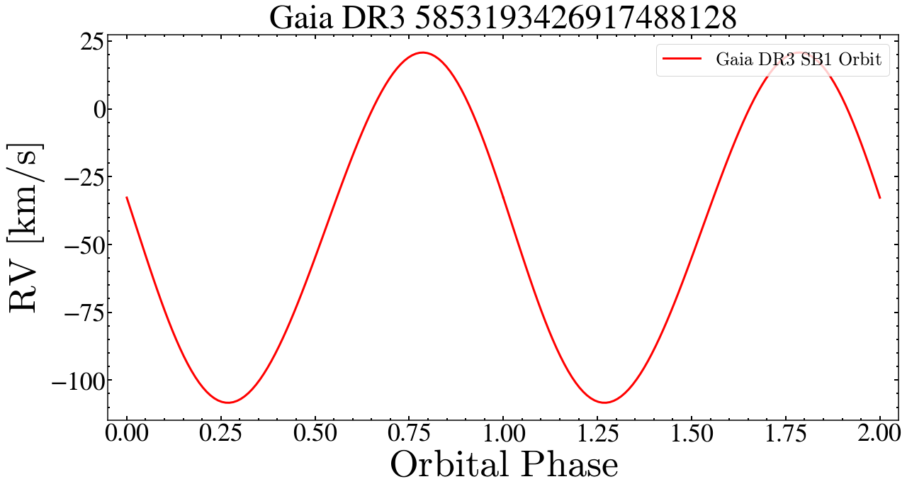

   

4. We can better understand the quality of the published orbit by looking at the published uncertainties. Draw from the published Gaia DR3 posteriors for the RV orbital parameters

   star.draw_from_sb1_model(draws=500)  

   Visualize the published orbit along with the 500 orbits drawn from the posteriors.

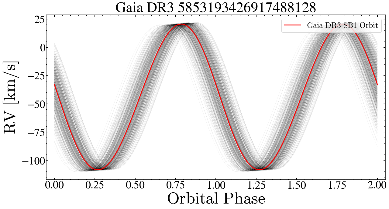
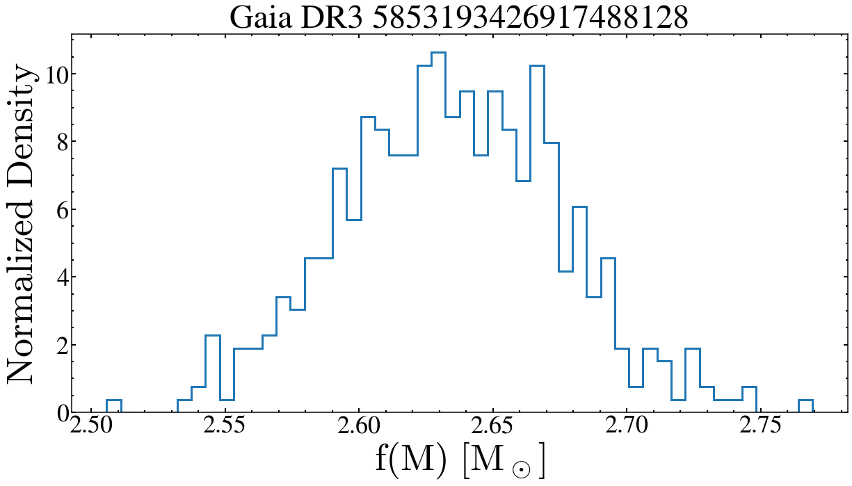
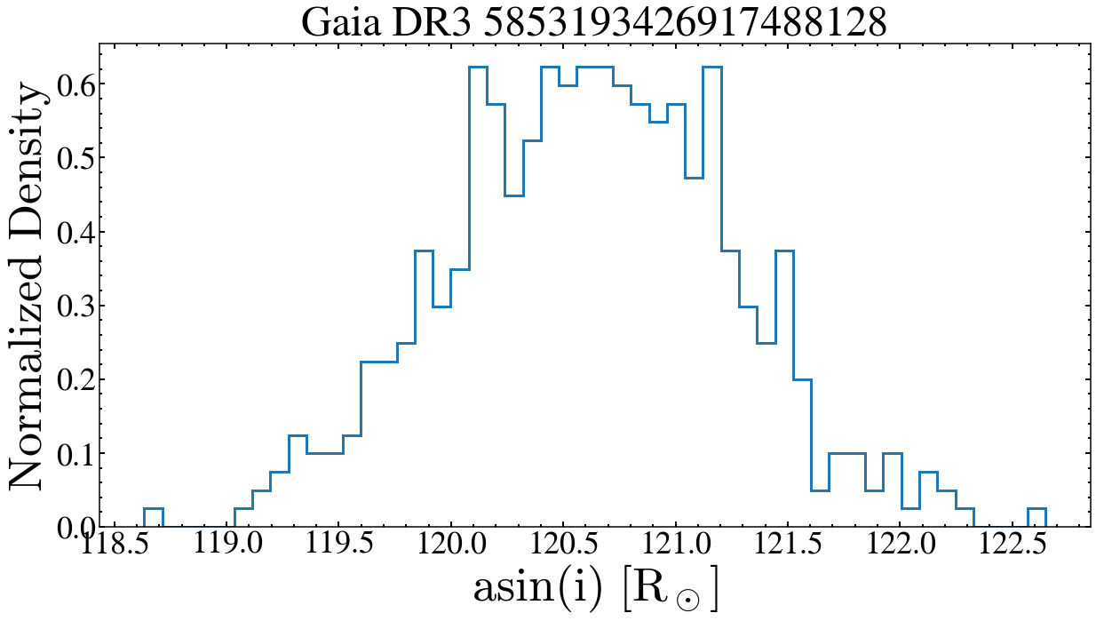
5. We can also look at the distribution of asini and f(M) for SB1 orbits.

   star.get_sb1_fm_dist()
   star.get_asini_dist() 
   
   print(f'f(M)={star.fm_50} +/- {star.fm_err} Msun')
   print(f'asini_1={star.asini1_50} +/- {star.asini1_err} Rsun')

7. If you are interested in targeting follow-up of the next RV min/max, this can also be handled:

   star.predict_next_rvminmax()
   print(f'Next RV maximum of {round(star.rv_max,1)} km/s will occur on JD={round(star.jd_next_rv_max,5)}.')     
   print(f'Next RV minimum of {round(star.rv_min,1)} km/s will occur on JD={round(star.jd_next_rv_min,5)}.')   

License

Distributed under the MIT License. See LICENSE.txt for more information.

(back to top)